Vegetation Mapping
 |
|
Introduction
With improvements in the resolution of remotely sensed data, data manipulation, storage facilities, and reduction in costs, the potential for producing a statewide vegetation map of North Carolina is now being realized. In cooperation with the North Carolina Natural Heritage Program (NCNHP), the North Carolina Center for Geographic Information and Analysis (CGIA), and the Multi-Resolution Land Characteristics Consortium (MRLC), NC-GAP has begun to map vegetation/landcover statewide. NC-GAP has the potential to serve as the linkage between ongoing landcover mapping efforts and ecologists & land managers in the creation of a high-quality vegetation layer for North Carolina.
As several states attempt vegetation mapping on this scale for the first time, these basic approaches are working:
NC-GAP is employing all these approaches to achieve the goal of mapping vegetation alliances throughout the state.
Ecological Boundaries
Due to the tremendous variation in vegetative communities across the state, we will develop vegetation maps within unique physiographic areas. We used the Ecological Units of the Eastern United States (Keys et. al 1995) developed by the US Forest Service to identify six distinct physiographic areas:
Initial Classification
NC-GAP has adopted the MRLC landcover map as an initial base layer for classification. The MRLC landcover map covers the northern portion of EPA Region IV and identifies fifteen (15) landcover catagories.
MRLC Landcover Classes:
NC-GAP will use the MRLC landcover map to mask out water (1), urban (2,3,4), agriculture (5,6), barren lands (13,14,15) and emergent wetlands (12) from the TM Imagery and work on classification of the remaining pixels. The adoption of the MRLC landcover map will save NC-GAP a great amount of time and effort that can be used to concentrate on the classification of the natural vegetative cover across the state. The MRLC landcover map also has the advantage of being developed for the entire southeast region, and could serve as an aid in edge matching the final vegetation maps from neighboring states that use it.
Airborne Videography
 |
From experience gained in Massachusetts, Florida,and Tennessee (Slaymaker et al. in prep., Pearlstine pers comm., Jones et al. 1995), videography has been proven to be a key in successfully mapping vegetation in the Eastern United States.
We stratified the state into physiographic regions (see above), and developed transect lines intersecting each region. We also made an effort to fly over significant stands of natural vegetation throughout the state. In addition, a set of videography transects for the three provinces of South Carolina were collected for SC-GAP. Flightlines covering the mountain province were carried over into Tennessee, Virginia, and Georgia to provide another data source for edge-matching efforts.
 Alexa setting up the dual video cameras |
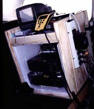 Video recorders and GPS setup in plane |
We're now using the video data for developing decision rules to map the vegetation. The method involved collecting continuous video transect data using two high-8mm cameras (Slaymaker et al., 1995). One camera is collecting data for a one-half kilometer swath and the other for a 30-meter swath "zoom", centered on the "wide".
A global positioning system (GPS) is used to collect positional data, and a "black box" encodes a time code directly on each video frame. After the flight is completed, the GPS data is differentially corrected and digitally related to the video time code.
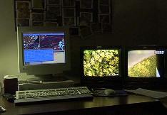 Interpretation station with video and TM imagery |
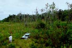 Collecting ground data in Brunswick Co. |
In the lab, the video data is converted to flightline coverages (with Arc/Info). The flightlines are displayed, along with road and hydrology coverages, over the raw or classified imagery. Nearby, the zoom and wide angle videos are displayed on two monitors. The time codes are used to determine the location of a point on the video and on the imagery (via the flightline coverages). Sites to be groundtruthed are selected, keeping accessibility in mind, and a snapshot of the site is taken with a video printer. Once in the field, a GPS unit is used to navigate to within 100 meters of the site and the video print is used to locate the site exactly.
The data collected at the site allows us to connect the appearance of tree canopies on the print with the representative species. The end result of the field data collection is a video print library, to aid in vegetation interpretation along all of the video transects. Once the video library is completed, the imagery along the video transect is interpreted, and vegetation classes are assigned. There is some spatial inaccuracy due to tip and tilt of the plane and limitations within the Arc/Info Grid module; therefore, interpretations are generally limited to homogeneous blocks of 25 pixels (5X5). After the video in interpreted for the study area, the data points are stratified by vegetation type and twenty-five percent (25%) are set aside for an accuracy assessment (to be performed after the map is thought to be stable).
The remaining seventy-five percent (75%) are then used to query the data layers used to model the vegetation. They include; National Wetland Inventories (NWI), Detailed Soil Surveys (NRCS), Digital Elevation Models (DEM), the clustered TM Imagery, and neighborhood functions (3x3) of the clustered TM Imagery (minimum, maximum, majority, diversity). The output of these queries are used to build decision rules for the image classification models.
After the decision rules have been written, the initial classification is perfomed, and the results are studied in conjunction with the interpreted video points and ancillary data sources. The decision rules are modified until a stable classification is reached. Accuracy assessment is then performed on the 25% of the data points not used in the decision rules.
Vegetation Classification System
The National Gap Analysis Program has set standards to be met by each state in the development of the databases (Scott, 1995). As a part of the setting of standards the program has supported the efforts of the Federal Geographic Data committee (FGDC) in the development of a standard vegetation classification (Jennings, 1993). The Southeast Regional Office of The Nature Conservancy is developing a portion of the National Vegetation Classification within the FGDC framework (Weakley et al, 1996). Below is one example of the hierarchy and how a plant alliance would be labeled.
Levels of Hierarchy:
| Level | Example | TNC Code |
|---|---|---|
| SYSTEM | Terrestrial | |
| PHYSIOGNOMIC CLASS | Forest | I |
| PHYSIOGNOMIC SUBCLASS | Deciduous forest | I.B |
| FORMATION GROUP | Cold-deciduous forest | I.B.2 |
| SUBGROUP | Natural/Semi-natural | I.B.2.N |
| FORMATION | Lowland or submontane cold-deciduous forest | I.B.2.N.a |
| ALLIANCE | Turkey Oak Forest | I.B.2.N.a.3 |
| ASSOCIATION | Turkey Oak/Little Bluestem forest |
To find out more, visit the National Vegetation Classification website (Adobe pdf format, 2686 kb).
The goal for GAP is to map the vegetation to the alliance level, the first level in which dominant species are identified. When the alliance level cannot be mapped due to limitations in the technology, data or level of effort required, we will identify supra-alliances which contain multiple alliances known to occur.