ABSTRACT
The Biodiversity and Spatial Information Center is modeling landscape scale changes to avian habitats based on various climate change scenarios within the South Atlantic Migratory Bird Initiative (SAMBI) geographic planning region. In coastal areas, the Sea Level Affecting Marshes Model (SLAMM) is being utilized to incorporate marsh migration dynamics due to longterm sea level rise (SLR). Inputs to SLAMM include National Wetlands Inventory (NWI) data cross-walked to 22 categories; a digital elevation model (DEM) with 30 meter resolution developed from the National Elevation Dataset (NED); slope derived from the DEM; an impervious surface data layer created for the National Land Cover Dataset (NLCD); tidal datum and sea level rise trend data from NOAA National Ocean Service's Center for Operational Oceanographic Products and Services (NOS/CO-OPS) stations.
The entire coastal extent (Atlantic and Gulf coasts) of the SAMBI was modeled with split processing using 39 USGS 8-digit Hydrologic Units Code (HUC) boundaries for coastal watersheds. NWI was rasterized from polygon data to a 30 meter cell size matching the NED DEM resolution. NWI was conflated with developed/urban classes within the Southeast Gap Analysis Project's land cover map and then cross-walked to 21 categories per SLAMM documentation (mangrove category excluded). Impounded or diked features were identified within the NWI and incorporated in modeling. Areas of inconsistent, erroneous, or systematically flawed data in the NED were identified visually and "fixed" using a variety of other data sources. Higher accuracy Light Detection and Ranging (LiDAR) elevation data were incorporated exclusively (i.e. in place of NED) for coastal regions in North Carolina because of the statewide availability of LiDAR. Tidal datum, present epoch (1983-2001) data and SLR trend data were downloaded from the NOAA NOS/CO-OPS website. Multiple stations may be located within any of the HUC boundaries along the SAMBI extent. Therefore, tidal datum data was used for the station whose values were closest to mean values for stations adjacent or within a HUC. Because not all stations have SLR trend information, data was taken from stations most proximal to a HUC.
The model was run using four climate scenarios (A1B, A2, B1, and A1FI) in 10 year increments for years 2000 to year 2100 using the "protect developed" option. Each of the 39 8-digit HUCs was run separately and then merged to create seamless decadel maps by climate scenario for coastal areas from southern Virginia to northern Florida.
INTRODUCTION
As part of the Designing Suitable Landscapes for Bird Species in the Eastern United States project, the Biodiversity and Spatial Information Center (BaSIC) is modeling landscape scale changes to habitat based on various climate change scenarios within the South Atlantic Migratory Bird Initiative (SAMBI) geographic planning region. Landscape change is being assessed using a combination of the USGS SLEUTH model for urban growth; vegetation dynamics using a spatially explicit stochastic state transition model (VDDT/TELSA) for ecological systems in the Southeast Gap Analysis (SE-GAP) Land Cover map; and sea level rise with the Sea Level Affecting Marshes Model (SLAMM) (Park et al. 1986). SLAMM attempts to simulate transforming coastal environments accounting for nearshore geomorphological processes such as accreation, erosion, and marsh migration dynamics due to longterm sea level rise. To this end, the SLAMM approach is much more robust than a non-dynamic "bathtub" model wherein an increase in ocean water levels simply inundates land.
METHODS
SLAMM Model Inputs
SLAMM was developed as a stand-alone program with a simple one form interface for Windows operating systems. The most recent version at the time BaSIC began modeling in the SAMBI extent was version 5.0.1 (Clough 2008). Six inputs are required to run SLAMM for a given geographic region:
- National Wetlands Inventory (NWI) data cross-walked to 21 categories (Table 1). A separate data layer for dikes/impoundments can be created from NWI to incorporate these features in modeling
- A digital elevation model (DEM)
- Slope derived from the DEM
- An impervious surface data layer
- Tidal datum information (usually obtained from NOAA National Ocean Service's Center for Operational Oceanographic Products and Services (NOS/CO-OPS) stations)
- Sea level rise (SLR) trend data (also obtained from NOAA NOS/CO-OPS stations)
USGS Hydrologic Unit Codes (HUCs)
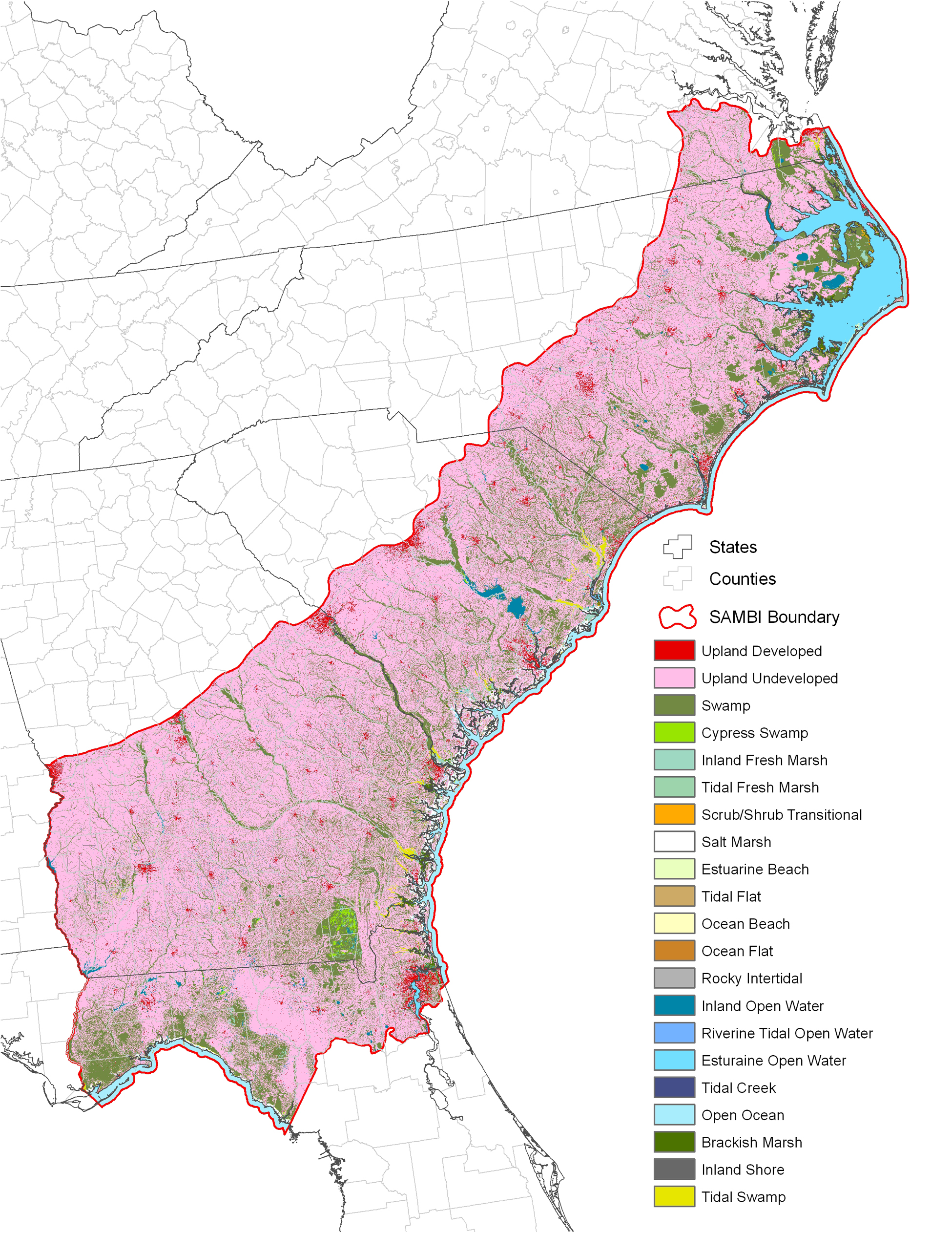
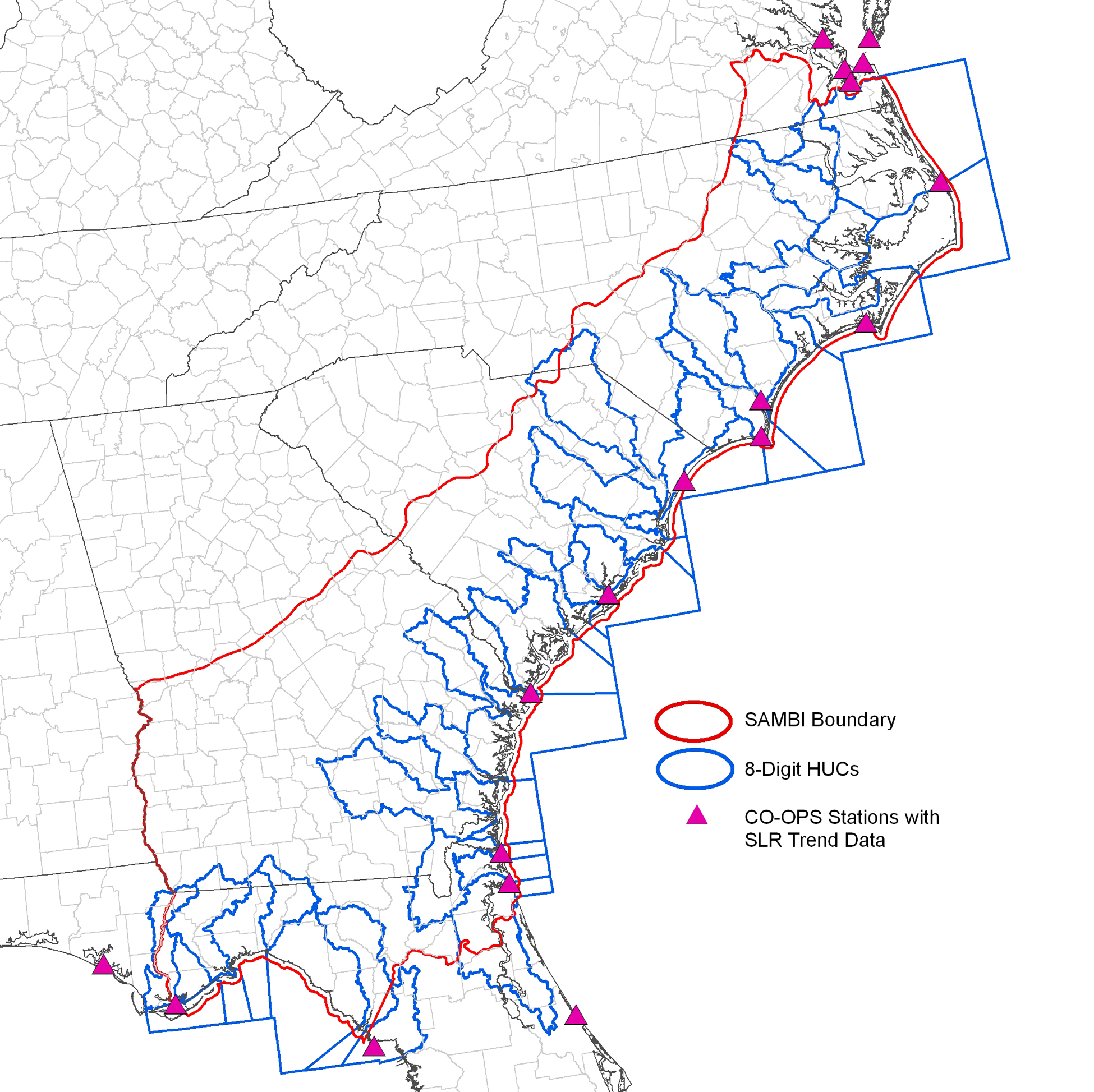
The HUC is part of a hierarchical classification system for surface water drainage in the US (Seaber et al. 1987). The numerical code represents a "cataloging unit" of delineation approximately larger than 1800 square kilometers. Within the SAMBI project boundary there are 39 coastal 8-digit HUCs (Figures 2 and 3). HUCs allow for partitioned processing when scripting complex spatial analysis tasks including SLAMM input data development as well as SLAMM modeling itself (see appendices at the end of this document).
National Wetlands Inventory
The NWI digital data of wetlands and deepwater habitats is produced by the United States Fish & Wildlife Service. Data production of polygons derived from aerial photograph interpretation began in 1977 in conjunction with the classification system developed by Cowardin et al. (1979). Generally, the Cowardin classification begins with marine, estuarine, riverine, lacustrine, and palustrine environments where coding starts with the first letter of each system (i.e. M, E, R, L, and P respectively). Subsequent portions of the code account for subsystem, class, subclass, and potentially up to four additional modifiers. For example, a polygon coded E1UB4L6 breaks down as follows:
|
E = estuarine system 1 = subtidal subsystem UB = unconsolidated bottom class |
4 = organic subclass L = subtidal water regime modifier 6 = oligohaline coastal halinity modifier |
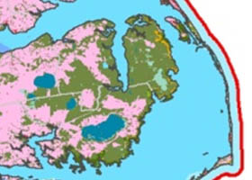
BaSIC compiled NWI data for the SAMBI and converted NWI polygons to rasters with cell values recoded to a 6-digit numeric system derived from the NWI code. This numeric code was then cross-walked to 21 categories according to SLAMM documentation (Table 1., Figure 1.) Developed Dry Land, and Undeveloped Dry Land categories (1 and 2 respectively) were extracted from the SE-GAP project land cover (see BaSIC documentation regarding this data layer). No NWI polygons included the estuarine intertidal forested/shrub scrub systems encompassing the Mangrove SLAMM category due to the SAMBI region extending only as far south as northern Florida.
An option in SLAMM allows for inclusion of dike features within the modeled extent. BaSIC modeling incorporated dikes as a separate data layer using NWI data coded with an "h" modifier.
Table 1. NWI- SLAMM cross-walk with descriptions.
| Raster Cell Code | SLAMM Category Name | NWI Code(s) | Description |
| 1 | DevDryland | U | Upland—Developed |
| 2 | UndDryland | U | Upland—Undeveloped, categories 1 & 2 need to be distinguished manually |
| 3 | Swamp | PFO, PFO1, PFO3-5, PSS, Ps | Palustrine forested (living or dead), and scrub shrub. Also, Palustrine forest and scrub-shrub with tidal influence. |
| 4 | CypressSwamp | PFO2 | needle-leaved deciduous |
| 5 | InlandFreshMrsh | L2EM, PEM[1&2] ["A"-"I"], R2EM | Lacustrine, Palustrine, and Riverine emergent |
| 6 | TidalFreshMarsh | R1EM, PEM["K"-"U"] | Riverine tidal emergent |
| 7 | Scrub Shrub / Transitional Marsh | E2SS1, E2FO | Estuarine intertidal scrub-shrub broad-leaved deciduous |
| 8 | Salt marsh | E2EM, [no "P"] | Estuarine intertidal emergent [won't distinguish high and low marsh]. |
| 9 | Mangrove | E2FO3, E2SS3 | Estuarine intertidal forested and scrub-shrub broad-leaved evergreen |
| 10 | Estuarine Beach | E2US2 or E2BB (PUS"K") | Estuarine intertidal unconsolidated shore sand or beach-bar, includes salt pans |
| 11 | TidalFlat | E2US[N,3,4,M], E2FL, M2AB, E2AB | Estuarine intertidal unconsolidated shore mud/organic or flat |
| 12 | Ocean Beach | M2US2, M2BB/UB/USN | Marine intertidal unconsolidated shore sand |
| 13 | OceanFlat | M2US3or4 | Marine intertidal unconsolidated shore mud or organic (Low energy coastlines) |
| 14 | RockyIntertidal | M2RS, E2RS, L2RS [E,M]2AB1[N,P] | Marine intertidal rocky shore |
| 15 | InlandOpenWater | R3-UB, R2-5OW L1-2OW, POW, PUB, R2UB, (L1-2,UB,AB) PAB, R2AB | Riverine, Lacustrine, and Palustrine open water and aquatic beds |
| 16 | RiverineTidalOpenWater | R1OW, R1RB, R1UB | Riverine tidal open water |
| 17 | EstuarineOpenWater | E1,(PUB"K" no "h") | Estuarine subtidal |
| 18 | TidalCreek | E2SB, E2UBN | Estuarine intertidal stream bed |
| 19 | OpenOcean | M1 | Marine subtidal |
| 20 | BrackishMarsh | E2EM[1-5]P | Irregularly Flooded Estuarine Intertidal Emergent |
| 21 | TallSpartina | N / A | 2M buffer automatically added to Salt Marsh fringe |
| 22 | InlandShore | L2UD, PUS, R[1..4]US/RS | shoreline not pre-processed using Tidal Range Elevations |
| 23 | TidalSwamp | PSS, PFO"K"-"V"/EM1"K"-"V" | Tidally influenced Swamp. |
| NOTE: NWI codes with an “h” modifier indicate diked/impounded areas | |||
Figure 1. NWI cross-walked to 21 SLAMM categories for the SAMBI extent.
Digital Elevation Model (DEM) - National Elevation Dataset
The USGS National Elevation Dataset (NED) consists of the most recent, highest quality data assembled for the United States at a spatial resolution of 30 meters (USGS 2003). However, because of the varying quality of the data, it was necessary to incorporate other datasets to create an improved, region wide product. These included data from NASA's Shuttle Radar Topography Mission (SRTM) at 30 meter resolution (NASA 2009), and hypsography data from the USGS's Digital Line Graphs (DLGs) at 1:24,000 and 1:100,000 scales (USGS 2009). Areas of inconsistent, erroneous, or systematically flawed data were identified visually and "tagged" for fixing. A number of algorithms were then used to reassign elevation values using interpolations based on the higher quality data. This essentially promoted the best available information for a given area using a number of sources, as opposed to re-interpolating data from the same flawed source.
The entire state of North Carolina has been mapped using Light Detection and Ranging (LiDAR) data from the North Carolina Floodplain Mapping Program (NCFMP 2009). Because the quality (precision, accuracy, and spatial resolution) is signicantly greater than the NED, BaSIC used only LiDAR derived elevations for the North Carolina portion of the SAMBI. These data were available at a 20 foot spatial resolution in a floating point decimal format and were resampled to 30 meters with a bilinear interpolation method (floating point decimal format was maintained).
Slope - derived from a digital elevation model
Slope is calculated from a DEM by determining the maximum rate of change (rise over run) between a given cell and its eight neighbors. Required input data format for SLAMM is slope measured in degrees.
Impervious Surface - National Land Cover Dataset
The National Land Cover Dataset (NLCD) was developed from LANDSAT Thematic Mapper satellite imagery to identify major categories of land use and cover throughout the United States at a resolution of 30 meters (Homer et al. 2004). Included during that development was a layer of impervious surface mostly representing urbanized areas. Each pixel was classified into 101 potential values (0-100%) based on reflectivity. Clusters of pixels with impervious surface percentages > 20% roughly correspond to human dominated environments. For SLAMM modeling, dry land with percent impervious > 25% is assumed to be "developed dry land."
Tidal Datum & Sea Level Rise Trend Information
SLAMM requires several parameter inputs compiled into a single text file (referred to in SLAMM documentation as a "site" file) with a specific format. Because the SAMBI was divided into 39 coastal HUCs to facilitate region wide processing, each HUC was a unique site with a unique input site file. Below is an example of a site file with appropriate formatting. The file (HUC3010107Site.txt) must include the "Site" text within the name:
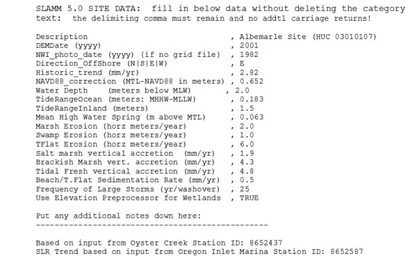
This file includes tidal datum information derived from NOAA NOS/CO-OPS stations located along coastal areas throughout the United States (including Alaska and Hawaii) (Figure 2). Data for the present epoch (1983-2001) is available online at the CO-OPS website .
Four input parameters utilized in SLAMM modeling are taken from measurements recorded at these stations:
- historic sea level rise trend
- NAVD88 datum correction
- ocean tide range
- mean high water spring
Historic SLR trend in mm/year is recorded directly at a handful of stations (Figure 3). That data is also available online from the NOAA NOS website .
The NAVD88 datum correction is calculated as the difference between two station measurements; MTL (mean tide level) and NAVD88 (North American Vertical Datum 1988) both measured in meters. Ocean tide range is calculated by subtracting MLLW (mean lower-low water) from MHHW (mean higher-high water). Mean high water spring is calculated by subtracting MTL (mean tide level) from MHW (mean high water).
Station latitude and longitude coordinates were used to a create point file. The station point file was intersected with HUC polygons to generate a file containing recorded measurements and HUC identification information. Because processing was done using 8-digit HUCs as unique sites and each HUC boundary contains multiple CO-OPS stations, it was necessary to normalize station measurements. Mean values for station measurements were calculated by HUC code and station data closest to those means were assigned to each HUC for site parameter inputs.
Figure 2. SAMBI extent, 8-Digit HUC boundaries, and NOS/CO-OPS station locations
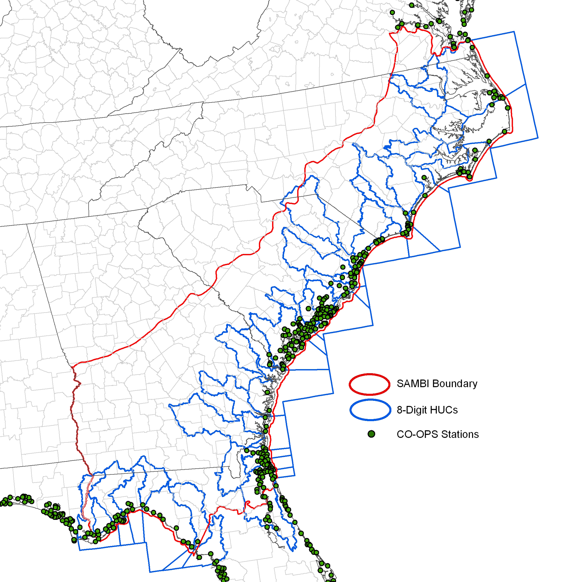
Figure 3. NOS/CO-OPS stations with sea level rise trend data within the SAMBI extent
All other parameter inputs were left as default values with exception of DEM date, NWI photo date, and direction offshore. DEM date was standardized as 2001 per NED data information. NWI photo date was established as 1982 since the majority of data within the SAMBI extent was collected during that year. Offshore direction was determined by visual inspection of each HUC's coastline boundary relative marine waters. Any of the input parameters specified in the site file can be changed by the user with additional site specific information.
SLAMM Data Input & Output Processing
All data layer inputs (NWI, DEM, slope, impervious surface, and dikes) for SLAMM are required to be in ASCII text format. File names for each input must be identical with the exception of the last three characters. These last three charcters are used by SLAMM to differentiate data:
- dem = DEM layer
- dik = dikes/impoundments layer
- imp = impervious surface layer
- nwi = NWI-SLAMM cross-walk layer
- slp = slope layer
For example, the site HUC 03010107 input file names would be as follows:
- Site file = HUC3010107Site.txt
- DEM file = HUC3010107dem.txt
- Dikes file = HUC3010107dik.txt
- Impervious suface file = HUC3010107imp.txt
- NWI-SLAMM cross-walk file = HUC3010107nwi.txt
- Slope file = HUC3010107slp.txt
Data were pre-processed and assembled in a raster environment and then converted to ASCII format using Arc Macro Language (AML) scripting (Appendix 1).
Model runs were automated using a VBScript that interacts with the SLAMM 5.0.1 Windows form interface (Appendix B). Models were run for four climate scenarios (A1B, A2, B1, and A1FI) in 10 year increments for years 2000 (initial conditions) to year 2100 using the "protect developed" option.
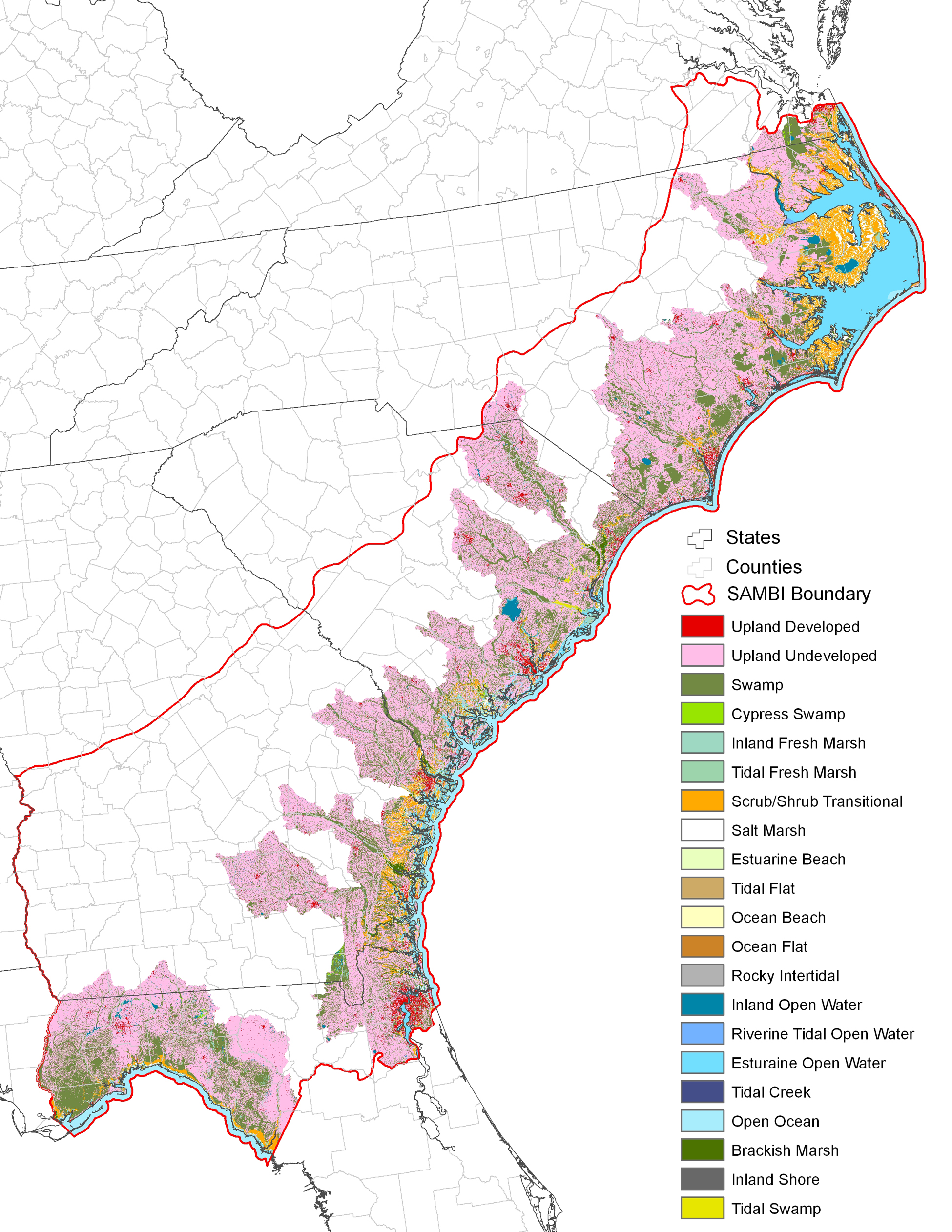
Outputs from SLAMM include ASCII raster text files and MS Excel spreadsheets for each climate scenario. To utilize model outputs in GIS, ASCII files were converted to ArcInfo GRID format. AML scripting was implemented to convert outputs to rasters and combine outputs (Appendices C and D). Each of the 39 8-digit HUCs was run separately and then merged to create seamless decadel maps by climate scenario for coastal areas from southern Virginia to northern Florida (Figures 4 and 5).
Figure 4. SLAMM output using climate scenario A1B for year 2000 (initial conditions) within the SAMBI extent
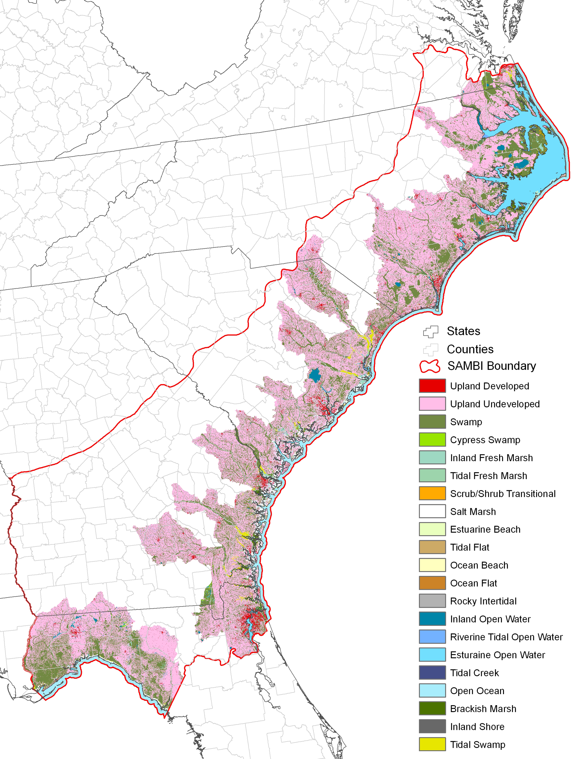
Figure 5. SLAMM output using climate scenario A1B for year 2100 within the SAMBI extent
AVAILABLE DATA
LITERATURE CITED
Clough, J. S. 2008. SLAMM 5.0.1. Technical documentation and executable program downloadable from http://www.warrenpinnacle.com/prof/SLAMM/index.html.
Cowardin, L. M. V. Carter, F. C. Golet, and E. T. LaRoe. 1979. Classification of wetlands and deepwater habitats of the United States. U.S. Dep. Interior, Fish and Wildl. Serv. FWS/OBS - 79/31.
Homer, C. C. Huang, L. Yang, B. Wylie and M. Coan. 2004. Development of a 2001 National Landcover Database for the United States. Photogrammetric Engineering and Remote Sensing, Vol. 70, No. 7, July 2004, pp. 829-840.
National Aeronautics and Space Administration. 2009. Jet Propulsion Laboratory, Califorinia Institute of Technology. Shuttle Radar Topography Mission. Available online, URL: http://www2.jpl.nasa.gov/srtm/.
North Carolina Floodplain Mapping Program. 2009. North Carolina Floodplain Mapping Information System. Available online, URL: http://www.ncfloodmaps.com/default_swf.asp?r=2.
Park, R. A., T. V. Armentano, and C. L. Cloonan. 1986. Predicting the Effects of Sea Level Ris on Coastal Wetlands. Pages 129-152 in J. G. Titus, ed. Effects of Changes in Stratospheric Ozone and Global Climate, Vol. 4: Sea Level Rise. U.S. Environmental Protection Agency, Washington, D.C.
Seaber, P.R., Kapinos, F.P., and Knapp, G.L., 1987, Hydrologic Unit Maps: U.S. Geological Survey Water-Supply Paper 2294, 63 p.
U.S. Geological Survey. 2003. National Mapping Division EROS Data Center. National Elevation Dataset. Available online, URL: http://ned.usgs.gov/.
U.S. Geological Survey. 2009. National Mapping Division EROS Data Center. Digital Line Graphs. Available online, URL: http://eros.usgs.gov/products/map/dlg.html.