INTRODUCTION
In the Southeastern U.S. rapid urbanization is a major challenge to developing long-term conservation strategies. The SAMBI DSL project used predicted urban growth models described herein to inform future landscape conditions that were also based climate change impacts and vegetative community succession. These future landscape conditions were then applied as a context for land use and management decisions in conservation planning.
SLEUTH, named for the model input datasets (Slope, Land use, Excluded, Urban, Transportation and Hillshade) is the evolutionary product of the Clarke Urban Growth Model that uses cellular automata, terrain mapping and land cover change modeling to address urban growth (Jantz et al, 2009; NCGIA 2011). SLEUTH provides urban growth projections which are useful across a range of applications; including wildlife habitat analysis, conservation planning, and land cover dynamics analysis. SLEUTH incorporates four growth rules (Spontaneous Growth, New Spreading Centers, Edge Growth and Road-Influenced Growth) to model the rate and pattern of urbanization. The model simulates not only outward growth of existing urban areas, but also growth along transportation corridors and new centers of urbanization. SLEUTH incorporates five parameters (Dispersion, Breed, Spread, Slope and Road Gravity) into the growth rules which project future urbanization. Possible parameter coefficient values range between 1 and 100. During calibration every possible combination of these five parameter coefficients (between defined start and stop values and by a defined step size) is applied to the growth rules, in order to find the combination that best matches past urbanization patterns observed in the training data. Once found, the model is run in prediction mode using these parameter values in the growth rules. The model produces one urban growth cycle per year. For each growth cycle, a GIF image is produced showing the probability of urbanization for each pixel.
This project utilized the SLEUTH-3r version of the model taking advantage of added new functionality and substantially increased performance (Jantz et al. 2009) over previous versions.
METHODS
Input Data
The input datasets for SLEUTH-3r were produced using the ESRI ArcGIS suite of geographic information systems software, with the exception of land use, which is optional for the model and was not used in this project. Slope was produced from the National Elevation Dataset (USGS, 2011) using the ESRI ArcGIS Slope tool from the Spatial Analyst Toolbox with the Percent Slope setting and a z-factor of 1. The z-factor is a multiplier used in cases where vertical units differ from horizontal units. Hillshade was produced from the NED raster data, (USGS, 2011), using the ESRI ArcGIS Hillshade tool from the Spatial Analyst Toolbox, with default settings.
The Excluded dataset provides a means for deterring future urbanization through weighted values. Possible exclusion values range from 1 to 100, where higher values indicate greater deterrent. The Excluded dataset was derived from the National Land Cover Dataset (MRLC 2001, Homer et al. 2007) and the Protected Areas Database of the US (PADUS, 2011). Areas classified as water in the 2001 NLCD were excluded from development entirely, as were beach and dune ecological systems in the 2001 Southeast Gap Analysis Project (SEGAP, 2011) land cover data. Wetland classes from 2001 NLCD were assigned a value of 95 because we assumed that only a small portion of wetlands would be developed. Additionally, areas with GAP status of 1-3 (indicating some form of permanent protection status) in PADUS were excluded entirely.
We modified the standard approach for developing urban and transportation input datasets. Prior studies have relied upon air photo interpretation and historical maps for delineation of these inputs (Dietzel, et al, 2004, Herold et al, 2003, NCGIA, 2011, Syphard et al, 2005). However, since this project has such an extensive study area, this approach was not feasible and an alternative was necessary. Line density analysis of roads from US Census Bureau TIGER Line Data (USCB, 2011a) was used to approximate prior urbanization. This approach was chosen due to the frequent and widely available nature of TIGER Line data. Through line density analysis of roads (excluding features such as un-paved roads and private drives), we were able to produce estimates of the urban extent for four input dates (2000, 2006, 2008 and 2009), incorporating exurban areas not classified as urban by regional land cover datasets such as NLCD, but which still impact wildlife habitat and habitat connectivity due to anthropogenic influence.
In order to implement this approach careful pre-processing of the roads coverage was necessary. Classification of road features was inconsistent, and in some areas roads such as private driveways and logging roads were classified as "Local, neighborhood, and rural road, city street, unseparated" (USCB, 2011a). As a result, in some areas, the estimations of urbanization for some input years were inflated, resulting in higher growth rates during calibration. Where this issue occurred roads with this classification which are also un-named were removed from consideration during the line density analysis. It was also discovered that in more recent versions of TIGER line data, divided highways were sometimes represented with a single feature per direction of travel where they had previously been represented with a single line feature representing all lanes of travel. Where this was observed, a similar inflation of growth rates in calibration occurred and undeveloped areas along interstates and divided state highways, etc. were more likely to be modeled as urbanized. In order to resolve this issue, major roads were buffered and centerlines were derived from the resulting polygons before line density analysis was performed.
TIGER Line data was also used in producing our transportation datasets. Strong inconsistencies exist within and between early versions of TIGER Line data. Highways and interstates exhibited the greatest thematic accuracy overall, and TIGER versions 2000 and more recent exhibited greatest positional accuracy. Road-Influenced Growth is most likely to occur along intestates and highways, not city or neighborhood streets where new roads and other components of urbanization appear simultaneously. Therefore, only interstates and highways were chosen to represent the transportation network. Because we already had compiled roads for use in developing our urban inputs, we chose to include the first and last dates of our urban inputs for our transportation datasets (2000 and 2009).
Study Area
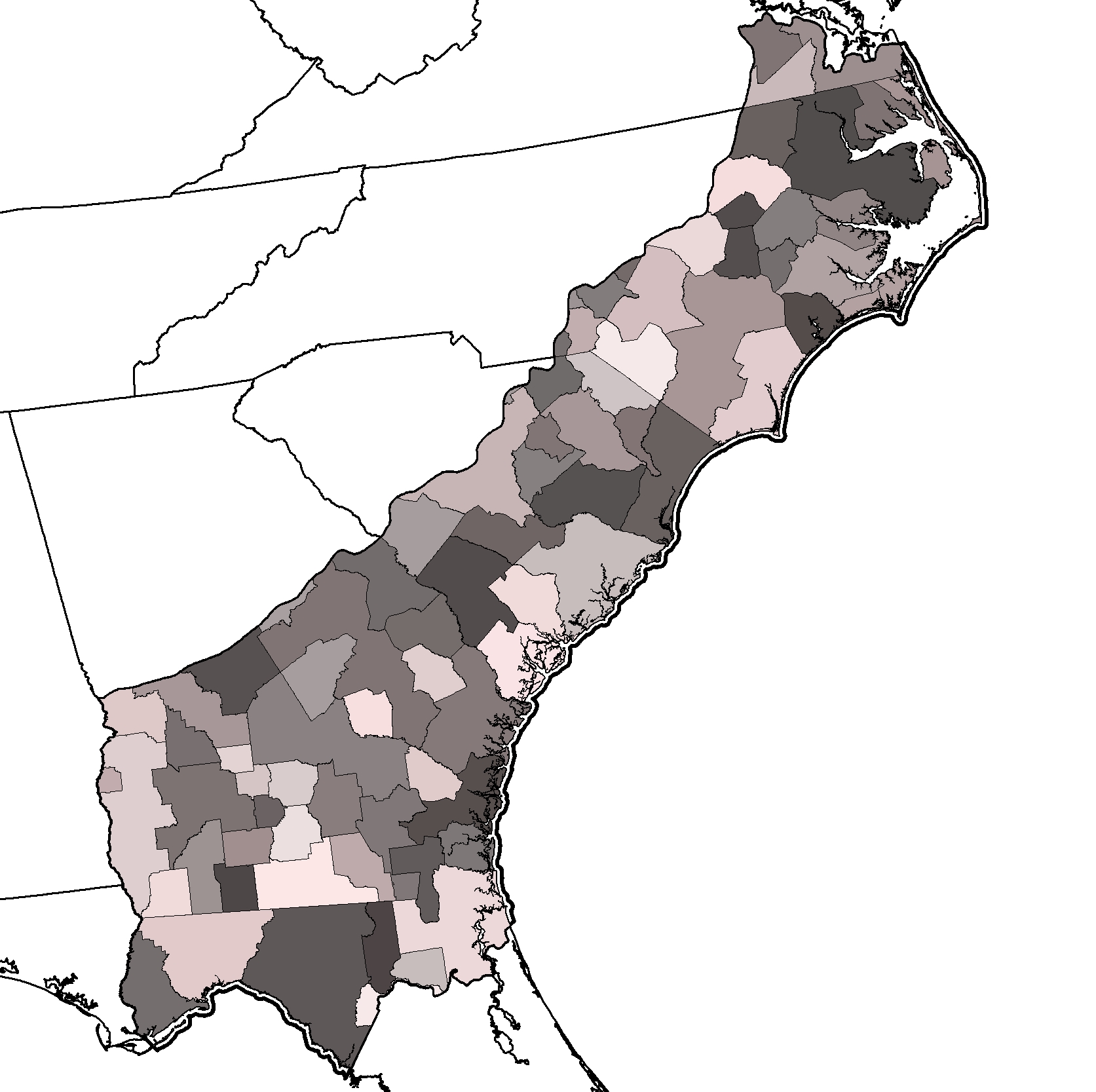
We developed input data for the entire South Atlantic Migratory Bird Initiative region (SAMBI), but subdivided the region for model calibration and prediction. The computationally demanding nature of SLEUTH3-r and the variability in growth rates and patterns throughout the region required the subdivision. We used the boundaries of US Census Bureau Combined Statistical Areas (CSA) as the basis for subdividing the SAMBI (Figure 1). A CSA is defined as two or more adjacent metropolitan or micropolitan statistical areas (with substantial commuting ties), each with a core area containing a substantial population nucleus and having a high degree of economic and social integration (USCB, 2011b). By conducting simulations across individual CSAs, we are maximizing the likelihood that our simulations occur across regions with uniform drivers of growth. We modified CSA boundaries for our simulations where they crossed state lines, and grouped counties not belonging to any CSA.
Figure 1. Aggregated US Census Bureau Combined Statistical Areas for SAMBI Extent
Code Changes
During testing of the SLEUTH3-r model with these datasets and sub-regions, we found the spreading growth it simulated was excessive and did not reflect prior growth patterns in the Southeast. We determined this was due to a setting in the model's spread.c file, which sets the number of neighboring urban pixels needed by a newly, spontaneously urbanized cell for it to become a new spreading urban center. Therefore, we increased the number of neighbors needed from the default of two to three in an eight cell neighborhood.
During calibration, the scenario file was altered in order to bypass Boom and Bust growth cycles. The Boom and Bust cycle was developed to replicate the tendency of growth to occur at non-linear rates with periods of greater and lesser growth (NCGIA, 2011). Both the upper and lower Boom and Bust values were set to 1 so that growth rate was not further affected when the growth rate fell below the Critical Low or exceeded the Critical High value. The Critical High and Critical Low values are thresholds to which the current cycle's growth rate is compared. If the growth rate falls below the Critical Low, slower growth is initiated by multiplying the growth rate by the Bust parameter (less than 1). If the growth rate exceeds the Critical High, faster growth is initiated by multiplying the growth rate by the Boom parameter (greater than 1).
Calibration
Previous studies have shown that, unlike the other four coefficients, the Road Gravity Coefficient does not exhibit a relationship to any fit statistic (Jantz et al, 2005). Due to its instability, this coefficient was fixed during both calibration and prediction phases of the model. The Road Gravity Coefficient was fixed at 100 principally because we only included interstates and highways in the transportation input datasets and reason that the most permissive coefficient value would best allow this transportation network to influence the mobilization of urbanization along it. Similarly, when modeling areas where slope is not a factor (e.g., the Coastal Plain), the Slope Coefficient was fixed at 25, with 0 being the most permissive coefficient value and 100 being the least permissive.
The first stage in calibration was to determine an initial Auxiliary Diffusion Multiplier (iADM) which, along with the diffusion coefficient and the number of pixels in the urban input image diagonal, determines the number of spontaneous urbanization attempts (Jantz et al, 2009). In order to determine the iADM, the Diffusion coefficient was set to 100 while all the others were set to their least permissive value. Twentyfive Monte Carlo simulations were performed in calibration mode. The area difference and ratio metrics were used to adjust the iADM until area was slightly over-estimated, similar to previous methods (Jantz et al, 2009). Once the iADM was determined, all coefficients were set to their most permissive to determine the maximum growth the model would predict with those coefficient values.
To conduct SLEUTH3-r calibration, metrics describing total area of urbanization, edge growth and number of clusters were compared between the input urbanization datasets and projections made by the model. In order to prevent any one of these three metrics from driving calibration disproportionately, we calculated and totaled the normalized error(s) in the three metrics. We chose the coefficient combinations with the least total error (within a tolerance of +/- 5% of observed to modeled Area) to drive subsequent calibration of the model coefficients until best single values were reached. Additionally, we adjusted the Auxiliary Diffusion Multiplier until the Dispersion coefficient was no longer forced to a minimum to produce least error. Calibration was run with 25 Monte Carlo simulations, using between 1 and 48 processors at the North Carolina State University High Performance Computing Center (NCSU HPC).
Prediction
Once near-optimal values were determined, the scenario file was edited for prediction. Best Fit Coefficient values were set, and Boom and Bust Parameters were each kept at 1 in order to reduce their influence on probability of urbanization projections. The near optimal values and calibration metrics are reported in Appendix A.
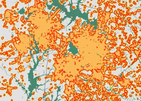
The colormap produced for output prediction images was altered in order to capture a 95% confidence interval for urbanization determined by the model. Prediction was run with 200 Monte Carlo simulations, using 48 processors on the NCSU HPC. Resulting output images represented the probability of urbanization at a 60 meter resolution. Where no probability of urbanization was predicted, the input hillshade is present as a backdrop to the image.
Post Processing
Post processing of the output images produced by the model converted them to ESRI grids .The hillshade background was removed in order to keep it from influencing any subsequent neighborhood or multiple-raster analyses. Output for all CSAs in the SAMBI were mosaiced and predicted growth was summarized across the SAMBI for each decadal time step. Annual outputs were archived and can be made available upon request to the Biodiversity and Spatial Information Center at NC State University ( www.basic.ncsu.edu ).
Updates
Modeling output for all CSAs in the Southeast Regional Assessment Project (Figure 2) were mosaiced and predicted growth was summarized for each decadal time step (Table 1). Because the SERAP modeling extent encompasses that of the SAMBI, separate downloads are not provided. After calibrations and predictions were completed for the SERAP, modeling was performed for the remaining portions of nearby US Department of Interior Landscape Conservation Cooperatives (Figure 3). As with the SAMBI, the entirety of each of the South Atlantic LCC and Peninsular Florida LCC is encompassed by the SERAP extent and separate downloads are not provided.
Figure 2. Aggregated US Census Bureau Combined Statistical Areas for SERAP Extent
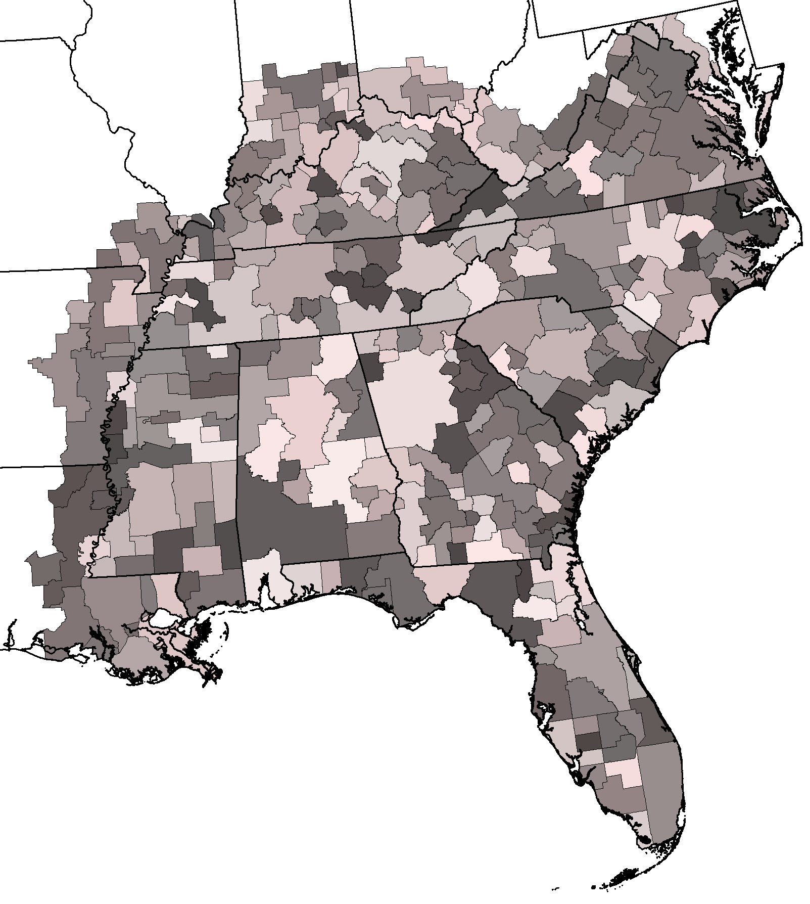
Table 1. SERAP Final Urban Growth Datasets
| File Name | Dataset Name | Year | |
| serap_sleuth.zip | serap_urb2010 | 2010 | |
| serap_sleuth.zip | serap_urb2020 | 2020 | |
| serap_sleuth.zip | serap_urb2030 | 2030 | |
| serap_sleuth.zip | serap_urb2040 | 2040 | |
| serap_sleuth.zip | serap_urb2050 | 2050 | |
| serap_sleuth.zip | serap_urb2060 | 2060 | |
| serap_sleuth.zip | serap_urb2070 | 2070 | |
| serap_sleuth.zip | serap_urb2080 | 2080 | |
| serap_sleuth.zip | serap_urb2090 | 2090 | |
| serap_sleuth.zip | serap_urb2100 | 2100 |
Figure 3. Additional modeling extents for Landscape Conservation Cooperatives
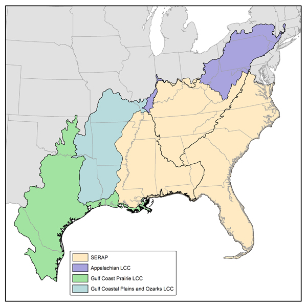
Table 2. Appalachian LCC Final Urban Growth Datasets
| File Name | Dataset Name | Year | |
| app_sleuth.zip | app_urb2020 | 2020 | |
| app_sleuth.zip | app_urb2030 | 2030 | |
| app_sleuth.zip | app_urb2040 | 2040 | |
| app_sleuth.zip | app_urb2050 | 2050 | |
| app_sleuth.zip | app_urb2060 | 2060 | |
| app_sleuth.zip | app_urb2070 | 2070 | |
| app_sleuth.zip | app_urb2080 | 2080 | |
| app_sleuth.zip | app_urb2090 | 2090 | |
| app_sleuth.zip | app_urb2100 | 2100 |
Table 3. Gulf Coast Prairie LCC Final Urban Growth Datasets
| File Name | Dataset Name | Year | |
| gcp_sleuth.zip | gcp_urb2020 | 2020 | |
| gcp_sleuth.zip | gcp_urb2030 | 2030 | |
| gcp_sleuth.zip | gcp_urb2040 | 2040 | |
| gcp_sleuth.zip | gcp_urb2050 | 2050 | |
| gcp_sleuth.zip | gcp_urb2060 | 2060 | |
| gcp_sleuth.zip | gcp_urb2070 | 2070 | |
| gcp_sleuth.zip | gcp_urb2080 | 2080 | |
| gcp_sleuth.zip | gcp_urb2090 | 2090 | |
| gcp_sleuth.zip | gcp_urb2100 | 2100 |
Table 4. Gulf Coastal Plains and Ozarks LCC Final Urban Growth Datasets
| File Name | Dataset Name | Year | |
| gcpo_sleuth.zip | gcpo_urb2020 | 2020 | |
| gcpo_sleuth.zip | gcpo_urb2030 | 2030 | |
| gcpo_sleuth.zip | gcpo_urb2040 | 2040 | |
| gcpo_sleuth.zip | gcpo_urb2050 | 2050 | |
| gcpo_sleuth.zip | gcpo_urb2060 | 2060 | |
| gcpo_sleuth.zip | gcpo_urb2070 | 2070 | |
| gcpo_sleuth.zip | gcpo_urb2080 | 2080 | |
| gcpo_sleuth.zip | gcpo_urb2090 | 2090 | |
| gcpo_sleuth.zip | gcpo_urb2100 | 2100 |
AVAILABLE DATA
LITERATURE CITED
Dietzel, C., K.C. Clarke. Spatial Differences in Multi-Resolution Urban Automata Modeling. Transitions in GIS; 2004, 8(4): 479-492
Herold, M., N.C. Goldstein, K.C. Clarke. The Spatiotemporal Form of Urban Growth: Measurement, Analysis and Modeling. Remote Sensing of Environment, 2003; 86: 286-302
Homer, C., Dewitz, J., Fry, J., Coan, M., Hossain, N., Larson, C., Herold, N., McKerrow, A., VanDriel, J.N., and Wickham, J. 2007. Completion of the 2001 National Land Cover Database for the Conterminous United States. Photogrammetric Engineering and Remote Sensing, Vol. 73, No. 4, pp. 337-341.
Jantz, C. A., S.J. Goetz. Analysis of scale dependencies in an urban land-use-change model. International Journal of Geographical Information Science; 2005, 19(2): 217-241
Jantz, C. A., S.J. Goetz, D. Donato and P. Claggett. Designing and Implementing a Regional Urban Modeling System Using the SLEUTH Cellular Urban Model. Computers, Environment and Urban Systems (2009), doi:10/1016/j.compenvurbsys.2009.08.03
Multi-Resolution Land Characteristics Consortium (MRLC); National Land cover Database 2001 (NLCD2001). http://www.mrlc.gov/about.php
National Center for Geographic Information Center and Analysis, University of California, Santa Barbara; Dept of Geography. http://www.ncgia.ucsb.edu/projects/gig/index.htmlProtected Areas of the United States. http://www.protectedlands.net/padus/
Southeast Gap Analysis Project Land cover Mapping Dataset. http://basic.ncsu.edu/segap/
Syphard, A.D., K.C. Clarke., J. Franklin. Using a Cellular Automaton Model to Forecast the Effects of Urban Growth on Habitat Pattern in Southern California. Ecological Complexity 2 (2005); 185-203United States Census Bureau Topologically Integrated Geographic Encoding and Referencing System. http://www.census.gov/geo/www/tiger/
United States Census Bureau. 2011. 2010 Census Summary File 1: 2010. Census of Population and Housing, Technical Documentation. http://www.census.gov/prod/cen2010/doc/sf1.pdf
U.S. Geological Survey. 2003. National Mapping Division EROS Data Center. National Elevation Dataset. Available online, URL: http://ned.usgs.gov/