INTRODUCTION
In the Southeastern U.S. rapid urbanization, climate change, and the direct and indirect impacts of those two dynamics on ecosystems are major challenges to developing long-term conservation strategies. In this project we modeled future landscape conditions under a variety of climate change scenarios in order to provide a context for land use and management decisions. To simulate vegetation dynamics, we used spatially explicit state-and-transition models and ESSA Technologies' Tool for Exploratory Landscape Scenario Analyses (TELSA; ESSA 2008a, ESSA 2008b, Kurz et al. 2000). Our vegetation dynamics projections were integrated with projected urban growth and sea level rise projections to develop the final dataset showing projected landscape conditions. Those projections were then used as input in the landscape prioritization decision support tools being developed at Auburn University.
METHODS
TELSA Modeling
There are four major inputs to TELSA: (1) a polygon map of vegetation types, (2) a non-spatial state-and-transition model for each vegetation type, (3) an initial age for each polygon, and (4) an initial structural stage for each polygon. The vegetation polygons are tracked through time with respect to their condition (state and stage) as a result of three general processes; succession, disturbance, and management. Succession is deterministic and disturbances are stochastic (e.g., fire, insect outbreak) processes are modeled.
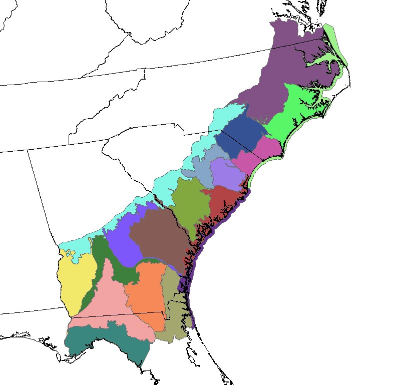
The SAMBI region was divided into 20 sub-regions based on Omernik Level IV ecoregion boundaries (U. S. EPA 2011), and vegetation dynamics were simulated across each sub-region separately (Figure 1). This was required due to computational limitations but also served as an additional hierarchical level within the modeling framework where transition parameters could be adjusted to reflect the local dynamics more precisely.
Figure 1. SAMBI Subregions Based on Omernik Level IV Ecoregions
Polygon Land Cover Map
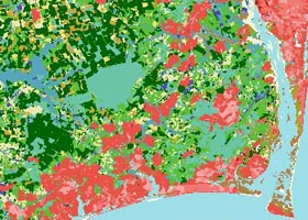
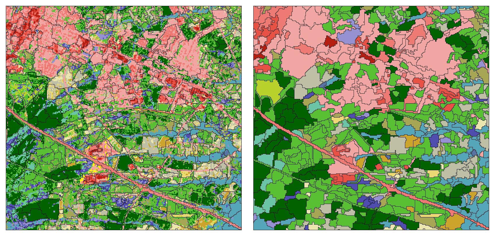
For each sub-region, polygons of land cover patterns were created using eCognition Elements 4.0 software (Definiens Imaging 2004) with a leaf on tassel-capped transformation of ca. 2001 Landsat TM imagery (Huang et al. 2002). The resulting polygons were then converted into a raster layer that maintained the unique ID of each polygon. Polygons were then attributed with the Southeast Gap Analysis Project (www.basic.ncsu.edu/segap/) ecological systems land cover type using a zonal majority function (Figure 2). A similar process was followed to attribute percent canopy cover and succession class from the LANDFIRE project (Rollins et al. 2008), and ownership (USGS National Gap Analysis Program 2008) to each polygon as well.
Figure 2. Reclass of Land Cover Polygons Using The Zonal Majority Function
State and Transition Models
The state-and-transition models we used were modified from the LANDFIRE Vegetation Dynamics Development Tool (VDDT) models (Smith et al. 2009). Those models had been developed in a series of regional workshops where ecologists familiar with the vegetation described the state and stage for each vegetation type and assigned probabilities of each disturbance (Figure 3). Each stage box has notation for class id, age range, sub-category id, and canopy closure class.
Figure 3. State-Transition Box Model
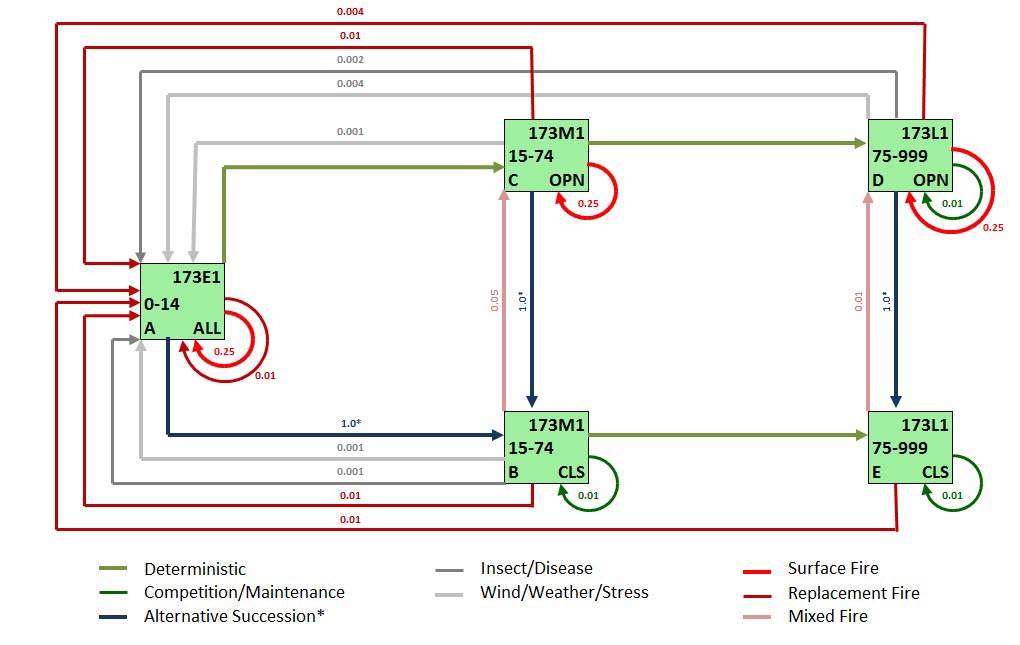
Some VDDT models have an Alternative Succession transition pathway. This pathway allows for an alternative to the deterministic transition of the ecological system under certain timeline and disturbance conditions. This pathway functions similarly to a deterministic pathway in that it has a probability of 1 and will occur if the specific time and disturbance criteria are met. In the Atlantic Coastal Plain example, an Alternative Succession pathway exists for a transition from box A (post replacement) to box B (mid-succession, closed canopy) if 10 years pass without any fire disturbance. If there is a fire, then it will take the polygon in the post replacement condition 14 years before transition to the mid succession, closed canopy condition. We developed two additional VDDT models to simulate the dynamics in publically and privately owned managed pine stands. In the SAMBI region, intensively managed pine stands (almost exclusively Loblolly Pine) are a major part of the forested landscape are readily identifiable on the landscape due to their conspicuous spectral signature and spatial pattern. The primary disturbance in these models is related to management activities (clearcuts, thinning, planting). We labeled these managed pine stands as public based on an overlay operation with the USGS Protected Areas Database layer. The difference between vegetation dynamics in publicly owned versus privately owned stands was a longer rotation time in the public lands.
One hundred forty of the 168 ecological systems and land use classes in the baseline land cover map (SEGAP citation) were modeled in TELSA for the SAMBI region. The remaining 20 classes were considered un-projectable because they were not ecological systems (e.g. water, agriculture) or did not have a LANDFIRE VDDT model associated with them. These classes were held constant throughout the model run and remained unchanged unless the polygons were converted to urban or inundated by sea level rise. State transition probabilities are provided for age and distrubance in Appendix A and Appendix B, respectively.
Climate Change Influence on Fire Regime
The vegetation dynamics models for the SAMBI incorporated the influence of projected climate change via changes to the fire regime. Time series regression was first used to estimate the relationship between climate and the amount of monthly acreage burned by wildfires. Monthly temperature and precipitation were used as predictors for both the current month's model estimate as well as observed temperature and precipitation for previous months to capture the long-term moisture budget. Once the parameters of the statistical model were estimated, empirically downscaled climate projections were used to project changes in the amount of acreage burned for a given CO2 emissions scenario. The uncertainty in the climate projections was quantified and propagated using model weights derived from Bayesian Model Averaging (BMA; Raftery et al. 2005; Bhat et al. 2011). The predictive variance for the probabilistic fire regime change projection was estimated using the Expectation Maximization algorithm (Dempster 1977) based on comparisons of the hindcast downscaled GCM output and the observed fire conditions. The predictive variance estimate was obtained by holding the GCM weights constant based on the BMA analysis. The modeled relationship was then used to project future wildfire frequencies under anticipated climate conditions projected by three emissions scenarios; A2, B1, A1B. The three climate scenarios represent a gradient of projected atmospheric CO2 levels and the associated effects of those levels on temperature and rainfall patterns. Changes in fire disturbance resulting from shifts in the climate would be reflected in the state and stage of vegetation. For example, increased fire disturbance would tend to keep systems subject to fire disturbance in an early succession stage.
Initial Age and State Class Assignment
Each polygon was assigned an initial ecological system label, age, succession class, and structure class. The ecological system, stage, and structure information were from the zonal majority operations described previously. An initial age for the polygons was assigned based on the US Forest Service FIA database forest type age distributions. The ecological systems were cross-walked to FIA forest types. A database query generated a proportional area for each age class in the FIA survey cycle whose date was closest to 2001. The area proportions were applied to the total area of each ecological system in each region thus establishing target areas for each age and ecological system combination. For each forest type, the ecological system polygons were randomly assigned an age value and the area of that polygon was added to that group's cumulative area total. This was repeated until the area target for that age and ecological system combination was reached. Provisions were made to ensure that ages were consistent with the implicit boundaries of the ecological systems succession stage and canopy cover (e.g., an early succession stand would not be assigned an age of 88 years).
The State Class ID that TELSA uses to model the polygons is a combination of an ecological system code, succession stage code (early [post-disturbance], mid, or late stage), and canopy structure code (early succession, closed, or open). The polygons were tracked with respect to their age and condition (state and stage) as a result of three general processes; succession, disturbance, and management.
Integration of Urban Growth and Sea Level Rise Model Output
After the map preparation and initial state class assignment, we used TELSA to simulate vegetation dynamics for 100 years for each climate scenario (2001-2100). Mapped output was generated at decadal time intervals. In a separate modeling effort, urban growth and sea level rise were simulated for the SAMBI region. These data layers were incorporated into the vegetation succession model output using zonal majority operations. Urban growth predictions took precedence over any transitions projected in the SLAMM output layers.
Urban growth projections were modeled independently with SLEUTH-3r model (Jantz et al, 2009) (see Urban Growth Modeling) and were used to identify vegetation polygons that were projected to transition from a vegetated to an urban cover type. Polygons were classified as urban if 50% or more of the pixels within the polygon had a greater than or equal to 50% probability of being converted to urban.
We incorporated sea level rise projections from Sea-Level Affecting Marshes Model (SLAMM; Clough 2008) (see Sealevel Rise Modeling) into the land cover maps independent of the TELSA modeling. For each TELSA output map, SLAMM data were used to reflect the conversion of land cover classes to alternate classes due to sea level rise projections. Each initial polygon was characterized with respect to the SLAMM data using a majority function. If the majority of the pixels within a vegetation polygon were "changed" pixels, the polygon was toggled to the appropriate class. When the transition had a one to one relationship with an ecological system, that system label was applied to the polygon. In some cases, there was a one-to-many relationship of a SLAMM class to ecological systems. In these cases, we used a spreadsheet script to analyze tables of adjacent polygons to determine the new ecological system label to apply to the SLAMM transformed polygons. If an adjacent polygon was labeled with an ecological system that satisfied the SLAMM crosswalk criteria, then the transformed polygon was assigned that label. Otherwise, the polygon was assigned the most common occurring related ecological system.
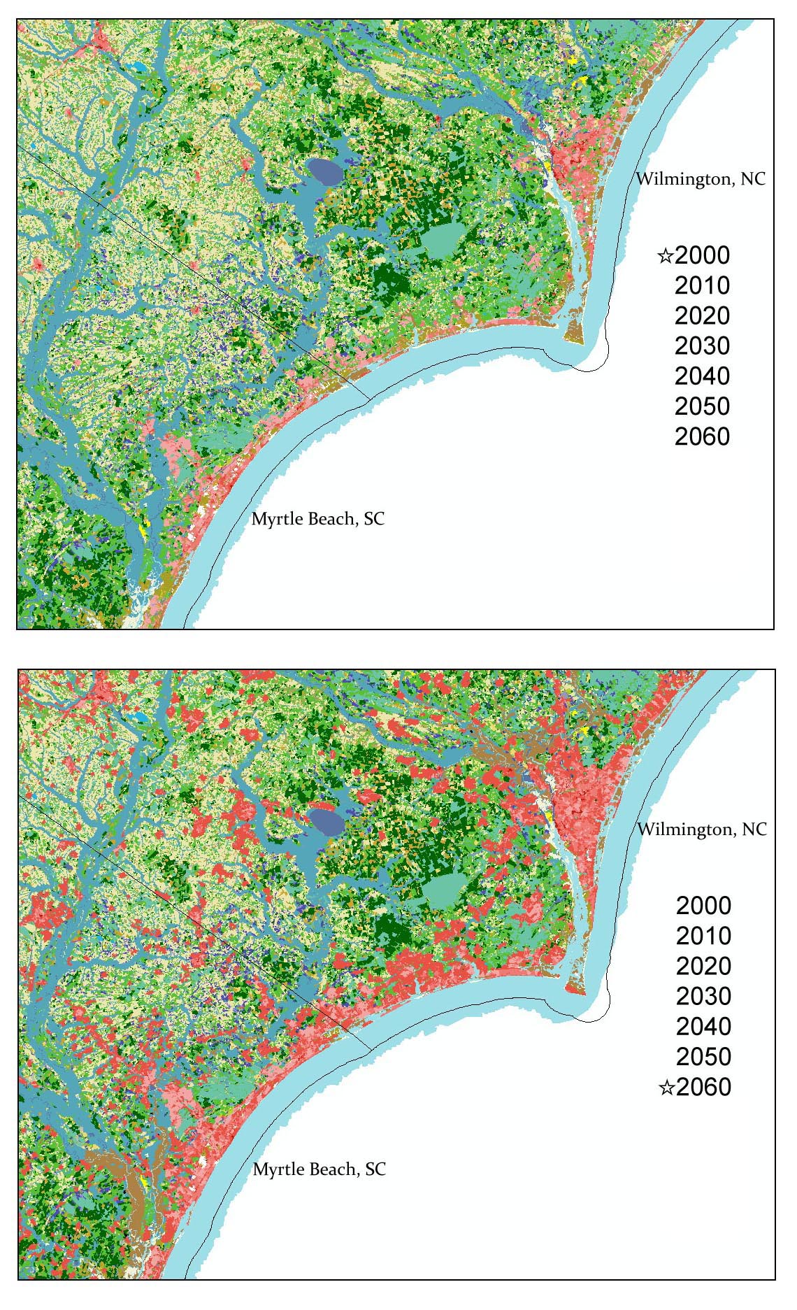
Figure 4. Integrated Land Cover Model Representing 2000 and 2060
Once the SLEUTH and SLAMM outputs had been integrated with the vegetation dynamics projections, the TELSA output tables were joined to the spatial data layers to create a grid for each 10 year time step. This was done for each of the climate scenarios by sub-region. The sub-region grids were then merged into one contiguous data layer for the SAMBI region.
AVAILABLE DATA
LITERATURE CITED
Bhat, S.K., M. Haran, A. Terando, R. Tonkonojenkov, and K. Keller, 2011: Climate projections using Bayesian model averaging and space-time dependence. Journal of Agricultural and Environmental Statistics, 16, 606-628.
Comer, P., D. Faber-Langendoen, R. Evans, S. Gawler, C. Josse, G. Kittel, S. Menard, M. Pyne, M. Reid, K. Schulz, K. Snow, and J. Teague. 2003. Ecological Systems of the United States: A Working Classification of U.S. Terrestrial Systems. NatureServe, Arlington, Virginia.
Clough, J. S. 2008. SLAMM 5.0.1. Technical documentation and executable program downloadable from http://www.warrenpinnacle.com/prof/SLAMM/index.html.
Definiens Imaging 2004. eCognition Elements Users Guide 4. Definiens Imaging GmbH, Munchen, Germany. 26 pp.
Dempster, A.P., N.M. Laird, and D.B. Rubin, 1977: Maximum likelihood from incomplete data via the EM algorithm. Journal of the Royal Statistical Society, 39B, 1-39.
ESSA Technologies Ltd. 2008a. TELSA: Tool for Exploratory Landscape Scenario Analyses, Model Description, Version 3.6. Vancouver, BC. 64 pp.
ESSA Technologies Ltd. 2008b. TELSA - Tool for Exploratory Landscape Scenario Analyses: User's Guide Version 3.6. Prepared by ESSA Technologies Ltd., Vancouver, BC. 235 pp.
Huang, C., B. Wylie, L. Yang, C. Homer, and G. Zylstra. 2002. Derivation of a tasseled cap transformation based on Landsat 7 at-satellite reflectance. International Journal of Remote Sensing, 23(8)1741-1748.
Jantz, C. A., S.J. Goetz, D. Donato and P. Claggett. Designing and Implementing a Regional Urban Modeling System Using the SLEUTH Cellular Urban Model. Computers, Environment and Urban Systems (2009), doi:10/1016/j.compenvurbsys.2009.08.03
Kurz,W.A., S.J. Beukema, W. Klenner, J.A. Greenough, D.C.E. Robinson, A.D. Sharpe, and T.M.Webb 2001. TELSA: The Tool for Exploratory Landscape Scenario Analyses.Computers and Electronics in Agriculture, Computers and Electronics in Agriculture 27(1-2) 227-242.
Raftery, A.E., T. Gneiting, F. Balabdaoui, and M. Polakowski, 2005: Using Bayesian model averaging to calibrate forecast ensembles. Monthly Weather Review, 133, 1155-1174.
Rollins, Matthew G.; Frame, Christine K., tech. eds. 2006. The LANDFIRE Prototype Project: nationally consistent and locally relevant geospatial data for wildland fire management. Gen. Tech. Rep. RMRS-GTR-175. Fort Collins: U.S. Department of Agriculture, Forest Service, Rocky Mountain Research Station. 416 p.
Smith, J., K. Blankenship, D. Johnson, S. Simon,C. Ryan, R. Swaty, M. Bucher, M. Brod and J. Patton. Adapting LANDFIRE Vegetation Dynamics Models. August 2009. Last accessed 24 April 2012 - http://www.conservationgateway.org/file/adapting-landfire-vegetation-dynamics-models].
U.S. Environmental Protection Agency. 2011. Level III and IV Ecoregions of the Conterminous United States. U.S. EPA Office of Research and Development. [Last accessed 24 April 2012 - http://www.epa.gov/wed/pages/ecoregions/level_iii_iv.htm#Level IV]
U.S.G.S. National Gap Analysis Program. 2008. Southeast GAP Regional Land Cover 2001. Biodiversity and Spatial Information Center, North Carolina Cooperative Fish and Wildlife Research Unit, NC State University (http://www.basic.ncsu.edu/segap/ last accessed 18 October 2010).